Goal
Build a machine learning model that predicts the probability that the first transaction of a new user is fraudulent.
import numpy as np
import pandas as pd
import seaborn as sns
import matplotlib.pyplot as plt
from sklearn.metrics import auc, roc_curve, classification_report

import h2o
from h2o.frame import H2OFrame
from h2o.estimators.random_forest import H2ORandomForestEstimator

%matplotlib inline
data = pd.read_csv('Fraud_Data.csv',parse_dates=['signup_time', 'purchase_time'])
1. Map users’ IP addresses to their countries
address2country = pd.read_csv('./IpAddress_to_Country.csv')
countries = []
for i in range(len(data)):
    ip_address = data.loc[i, 'ip_address']
    tmp = address2country[(address2country['lower_bound_ip_address'] <= ip_address) &
                          (address2country['upper_bound_ip_address'] >= ip_address)]
    if len(tmp) == 1:
        countries.append(tmp['country'].values[0])
    else:
        countries.append('NA')

data['country'] = countries
data.head()
| user_id | signup_time | purchase_time | purchase_value | device_id | source | browser | sex | age | ip_address | class | country | |
|---|---|---|---|---|---|---|---|---|---|---|---|---|
| 0 | 22058 | 2015-02-24 22:55:49 | 2015-04-18 02:47:11 | 34 | QVPSPJUOCKZAR | SEO | Chrome | M | 39 | 7.327584e+08 | 0 | Japan |
| 1 | 333320 | 2015-06-07 20:39:50 | 2015-06-08 01:38:54 | 16 | EOGFQPIZPYXFZ | Ads | Chrome | F | 53 | 3.503114e+08 | 0 | United States |
| 2 | 1359 | 2015-01-01 18:52:44 | 2015-01-01 18:52:45 | 15 | YSSKYOSJHPPLJ | SEO | Opera | M | 53 | 2.621474e+09 | 1 | United States |
| 3 | 150084 | 2015-04-28 21:13:25 | 2015-05-04 13:54:50 | 44 | ATGTXKYKUDUQN | SEO | Safari | M | 41 | 3.840542e+09 | 0 | NA |
| 4 | 221365 | 2015-07-21 07:09:52 | 2015-09-09 18:40:53 | 39 | NAUITBZFJKHWW | Ads | Safari | M | 45 | 4.155831e+08 | 0 | United States |
2. Feature Engineering
#check time difference between purchase and register
time_diff = data['purchase_time'] - data['signup_time']
time_diff = time_diff.apply(lambda x: x.seconds)
data['time_diff'] = time_diff

# Check user number for unique devices
device_num = data[['user_id', 'device_id']].groupby('device_id').count().reset_index()
device_num = device_num.rename(columns={'user_id': 'device_num'})
data = data.merge(device_num, how='left', on='device_id')
ip_num = data[['user_id', 'ip_address']].groupby('ip_address').count().reset_index()
ip_num = ip_num.rename(columns={'user_id': 'ip_num'})
data = data.merge(ip_num, how='left', on='ip_address')
data['signup_day'] = data['signup_time'].apply(lambda x: x.dayofweek)
data['signup_week'] = data['signup_time'].apply(lambda x: x.week)

# Purchase day and week
data['purchase_day'] = data['purchase_time'].apply(lambda x: x.dayofweek)
data['purchase_week'] = data['purchase_time'].apply(lambda x: x.week)
columns = ['signup_day', 'signup_week', 'purchase_day', 'purchase_week', 'purchase_value', 'source',
           'browser', 'sex', 'age', 'country', 'time_diff', 'device_num', 'ip_num', 'class']
data = data[columns]
3. Build Random Forest Model with H2O Frame
# Initialize H2O cluster
h2o.init()
h2o.remove_all()

# Transform to H2O Frame, and make sure the target variable is categorical
h2o_df = H2OFrame(data)

for name in ['signup_day', 'purchase_day', 'source', 'browser', 'sex', 'country', 'class']:
    h2o_df[name] = h2o_df[name].asfactor()
# Split into 70% training and 30% test dataset
strat_split = h2o_df['class'].stratified_split(test_frac=0.3, seed=42)

train = h2o_df[strat_split == 'train']
test = h2o_df[strat_split == 'test']

# Define features and target
feature = ['signup_day', 'signup_week', 'purchase_day', 'purchase_week', 'purchase_value',
           'source', 'browser', 'sex', 'age', 'country', 'time_diff', 'device_num', 'ip_num']
target = 'class'
# Build random forest model
model = H2ORandomForestEstimator(balance_classes=True, ntrees=100, mtries=-1, stopping_rounds=5,
                                 stopping_metric='auc', score_each_iteration=True, seed=42)
model.train(x=feature, y=target, training_frame=train, validation_frame=test)
Checking whether there is an H2O instance running at http://localhost:54321 ..... not found.
Attempting to start a local H2O server...
  Java Version: openjdk version "15.0.2" 2021-01-19; OpenJDK Runtime Environment (build 15.0.2+7); OpenJDK 64-Bit Server VM (build 15.0.2+7, mixed mode, sharing)
  Starting server from /opt/anaconda3/lib/python3.8/site-packages/h2o/backend/bin/h2o.jar
  Ice root: /var/folders/yf/vgp_y5cn7c79tm73jsfjm3k00000gn/T/tmpchdaa8vj
  JVM stdout: /var/folders/yf/vgp_y5cn7c79tm73jsfjm3k00000gn/T/tmpchdaa8vj/h2o_mia_started_from_python.out
  JVM stderr: /var/folders/yf/vgp_y5cn7c79tm73jsfjm3k00000gn/T/tmpchdaa8vj/h2o_mia_started_from_python.err
  Server is running at http://127.0.0.1:54321
Connecting to H2O server at http://127.0.0.1:54321 ... successful.
| H2O_cluster_uptime: | 02 secs |
| H2O_cluster_timezone: | America/Los_Angeles |
| H2O_data_parsing_timezone: | UTC |
| H2O_cluster_version: | 3.32.1.6 |
| H2O_cluster_version_age: | 17 days |
| H2O_cluster_name: | H2O_from_python_mia_ykfcn6 |
| H2O_cluster_total_nodes: | 1 |
| H2O_cluster_free_memory: | 4 Gb |
| H2O_cluster_total_cores: | 12 |
| H2O_cluster_allowed_cores: | 12 |
| H2O_cluster_status: | accepting new members, healthy |
| H2O_connection_url: | http://127.0.0.1:54321 |
| H2O_connection_proxy: | {"http": null, "https": null} |
| H2O_internal_security: | False |
| H2O_API_Extensions: | Amazon S3, XGBoost, Algos, AutoML, Core V3, TargetEncoder, Core V4 |
| Python_version: | 3.8.8 final |
Parse progress: |█████████████████████████████████████████████████████████| 100%
drf Model Build progress: |███████████████████████████████████████████████| 100%
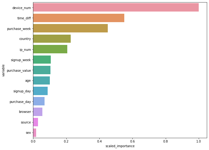
4. Show the feature importance
# Feature importance
importance = model.varimp(use_pandas=True)

fig, ax = plt.subplots(figsize=(10, 8))
sns.barplot(x='scaled_importance', y='variable', data=importance)
plt.show()
# Make predictions
train_true = train.as_data_frame()['class'].values
test_true = test.as_data_frame()['class'].values
train_pred = model.predict(train).as_data_frame()['p1'].values
test_pred = model.predict(test).as_data_frame()['p1'].values

train_fpr, train_tpr, _ = roc_curve(train_true, train_pred)
test_fpr, test_tpr, _ = roc_curve(test_true, test_pred)
train_auc = np.round(auc(train_fpr, train_tpr), 3)
test_auc = np.round(auc(test_fpr, test_tpr), 3)
drf prediction progress: |████████████████████████████████████████████████| 100%
drf prediction progress: |████████████████████████████████████████████████| 100%
# Classification report
print(classification_report(y_true=test_true, y_pred=(test_pred > 0.5).astype(int)))
              precision    recall  f1-score   support

           0       0.95      1.00      0.98     41088
           1       1.00      0.53      0.69      4245

    accuracy                           0.96     45333
   macro avg       0.98      0.76      0.83     45333
weighted avg       0.96      0.96      0.95     45333
Explanation
class = 0 : not fraudulent
class = 1 : fraudulent
recall = 0.53 for class 1, meaning this model can only detect 53% of all fraudulent activities.
precision = 0.95 for class 0 , meaning 95% the non-fraudulent activities defined by this model are real non-fraudulent activities.
The reason why recall rate is low for fraudulent class is that the cut-off point is default to be 0.5. So I may lower the cut-off point to see the recall change.
# Classification report
print(classification_report(y_true=test_true, y_pred=(test_pred > 0.05).astype(int)))
              precision    recall  f1-score   support

           0       0.97      0.95      0.96     41088
           1       0.58      0.67      0.62      4245

    accuracy                           0.92     45333
   macro avg       0.77      0.81      0.79     45333
weighted avg       0.93      0.92      0.93     45333
Explanation
The recall value of fraudulent class increased to 0.67 after decreasing cut-off point from 0.5 to 0.05.
However, other metrics performs worse than before.
For example, the precision for fraudulent class decreased from1 to 0.58, meaning that 57% of the detedt fraudulent are real fraudulent activities.
A lower presicion obviously is not what I want, so for further research, hyperparatemer cut-off point should be tuned subtily for best classification.
Here is a way to evaluate the model’s classification ability, which are ROC curve and AUC value.
train_fpr = np.insert(train_fpr, 0, 0)
train_tpr = np.insert(train_tpr, 0, 0)
test_fpr = np.insert(test_fpr, 0, 0)
test_tpr = np.insert(test_tpr, 0, 0)

fig, ax = plt.subplots(figsize=(8, 6))
ax.plot(train_fpr, train_tpr, label='Train AUC: ' + str(train_auc))
ax.plot(test_fpr, test_tpr, label='Test AUC: ' + str(test_auc))
ax.plot(train_fpr, train_fpr, 'k--', label='Chance Curve')
ax.set_xlabel('False Positive Rate', fontsize=12)
ax.set_ylabel('True Positive Rate', fontsize=12)
ax.grid(True)
ax.legend(fontsize=12)
plt.show()
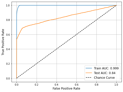
5. Conclusion
The Test AUC score is 0.85.
Normally for test AUC score 0.7 to 0.8 is considered acceptable, 0.8 to 0.9 is considered excellent.
So this cluster is excellent for detecting fraudulent activities.
h2o.cluster().shutdown()